一、前言
- 环境介绍
- 系统:win10
- 语言:python3.7
- 框架:pytorch1.1
- 内容概要
- 神经网络分类实验(对应于机器学习的聚类算法Kmeans)
- 手写数字集识别(神经网络+工程)
二、神经网络对数据分类
2.1 网络数据生成
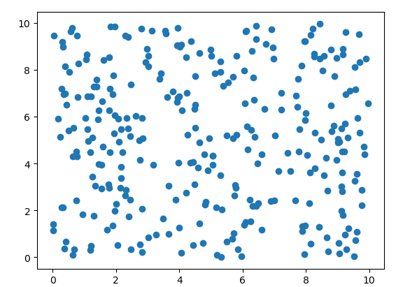
- 步骤一:
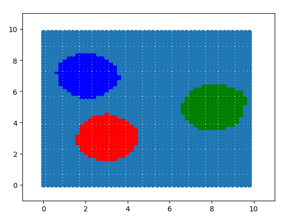
先随机生成一些数据,数据截图如下:
- 步骤二
通过两个相交的函数将数据分为4类,分类结果如下:
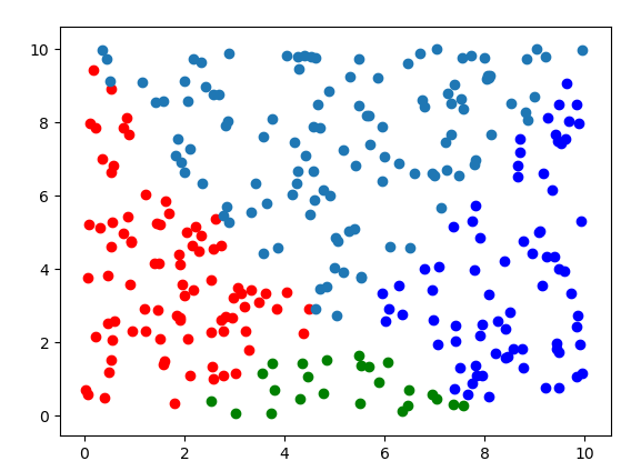
分割函数如下设计:
代码如下:1
2
3
4
5
6
7
8
9
10
11
12
13
14
15
16
17
18
19
20
21
22
23
24
25
26
27
28
29
30
31
32
33
34
35
36
37
38
39
40
41
42
43
44
45class TrainData(data.Dataset):
def __init__(self):
super(TrainData,self).__init__()
self.TrainData = self.generateTrainData()
def __getitem__(self, item):
return torch.Tensor(self.TrainData[item,0:2]), torch.Tensor([self.TrainData[item, 2]])
def __len__(self):
return len(self.TrainData)
def generateTrainData(self):
outData = []
centerPoint = [[3,3],[8,5],[2,7]]
for i in range(300):
rand_x = np.random.random_sample(1)[0] * 10
rand_y = np.random.random_sample(1)[0] * 10
# label = 3
# for index,(x,y) in enumerate(centerPoint):
# if np.sqrt(np.power(rand_x - x,2) + np.power(rand_y-y,2)) <= 1.5:
# label = index
x1 = 0.1 * np.power(rand_x, 2)
x2 = 0.1 * np.power(rand_x - 10, 2)
if (rand_y <= x2) and (rand_y >= x1):
label = 0
elif (rand_y <= x2) and (rand_y <= x1):
label = 1
elif (rand_y >= x2) and (rand_y <= x1):
label = 2
else:
label = 3
outData.append([rand_x, rand_y, label])
outData = np.array(outData)
plt.scatter(outData[outData[:, 2] == 0, 0], outData[outData[:, 2] == 0, 1], c="r")
plt.scatter(outData[outData[:, 2] == 1, 0], outData[outData[:, 2] == 1, 1], c="g")
plt.scatter(outData[outData[:, 2] == 2, 0], outData[outData[:, 2] == 2, 1], c="b")
plt.scatter(outData[outData[:, 2] == 3, 0], outData[outData[:, 2] == 3, 1])
plt.show()
return outData
2.2 网络设计
网络分为4层,为什么要4层!!随意吧,反正越多效果越好,越多学习速率越慢。网络层数3层也行,重要是激励函数,激励函数我使用了4种:
- 无激励函数:函数学习速度快,但是不理想,因为没有激励函数,输出只不过是输入的线性组合,发挥不出网络的威力。
- Sigmoid激励函数:按道理这里应该使用
Sigmoid或者softmax激励函数,他们的输出都是0~1,适合用于处理分类问题(逻辑回归),但是这里为了熟悉线性回归,使用了以下两个激励函数,可以看出需要的神经元数量还是相当的多。 - relu激励函数:学习速度快,学习的结果不错。他和无激励函数的区别就是它可以选择性的使得一些神经元失去活性,更加类似于人的大脑。函数表示为:
return max(x,0) - Softplus激励函数:学习速度略慢与relu,学习结果比relu更加圆滑。数学表达式为:$log(1+e^x)$
既然relu和Softplus都可以,选择就出现了。如果面对比较深的网络选择使用relu,浅的网络选择使用Softplus。
1 | class net(nn.Module): |
2.3 训练数据
1 | def setparamsLr(model,lr): # 修改学习速率 |
2.4 测试结果
测试代码
1 | module.eval() |
从下图可以看出,学校效果不错
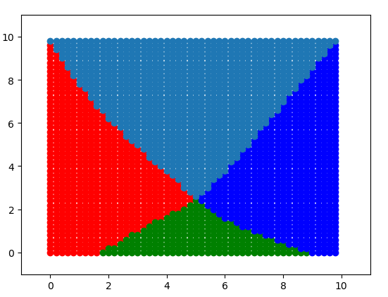
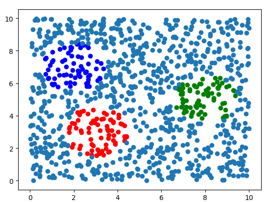
再随机生成一些数据,测试网络
2.5 思考
神经网络分类的网络搭建和神经网络拟合在设计上面的区别
三、卷积神经网络
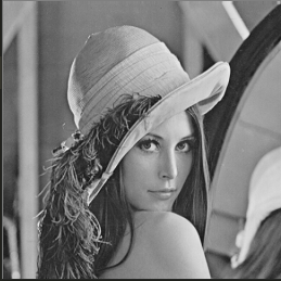
这里不讲图片卷积的基础原理,推荐看《数字图像处理》——冈萨雷斯。本章以对图片去噪为例子。
3.1 传统去噪方法
这里使用椒盐噪声为例,什么是椒盐噪声,就是图片上面被纯黑色和纯白色干扰的图片。
原图片如下:
加上椒盐噪声:

使用中值滤波器滤波之后:

仿真代码如下:
1 | import numpy as np |
好像并不能很好的解释卷积,不管了,沾到一点边即可。
3.2 神经网络去噪方法
主要步骤如下:
- 数据集(由于搜集数据集太过麻烦,所以。。。)
- 网络设计(设计一个隐藏层就好)
- 损失函数设计(应该没有自带的损失函数了)
开始实现:
具体:略
四、手写数字集实现
已经写过了,详情请参考以下内容:
主要步骤如下:
- 数据集(官方有,pytorch直接通过网络下载)
- 网络设计(使用成熟的2层卷积网络,3层线性网络,这是成熟的google网络好像)
- 损失函数设计(使用自带的交叉损失函数)
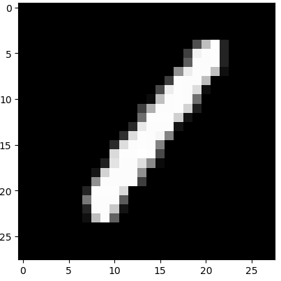
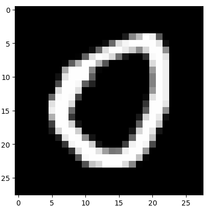
4.1 数据集
1 | import torchvision |
查看数据集代码:1
2
3
4
5
6import matplotlib.pyplot as plt
for D,L in train_data:
print(L[0])
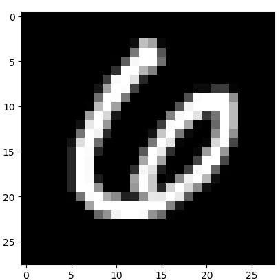
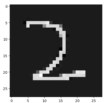
print(D[0][0])
plt.imshow(D[0][0],cmap="gray")
plt.show()
训练数据截图
4.2 网络设计
这里使用的是现有的网络模型LeNet1 ,注意每一层的输出尺寸,容易写错。
1 | import torch.nn as nn |
4.3 开始训练并测试
1 | from torch.utils.data import DataLoader |
运行,从打印结果可以看出,准确率可以达到98%左右。
五、制作手写窗口
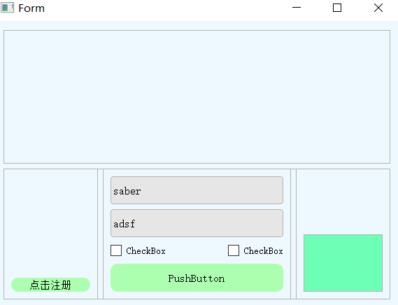
第四章写的是学习手写数字,这一章写应用,目标设计如下图所示:
5.1 程序结构
整个程序设计分为三个部分:
- 界面设计(略讲,我也不懂)
- 画板功能实现
- 重写widget内的paintEvent函数
- 图层管理
- 按键功能实现(信号与槽)
- 界面排版
- 界面渲染
- 画板功能实现
- 图像分割
- 简单分割
- 获取X坐标
- 获取Y坐标
- 添加Padding(因为训练集有Padding,没办法)
- 精确分割
- 图像二值化
- 宽度优先遍历
- 深度优先遍历
- 简单分割
- 图像识别
- 数据集获取
- 网络搭建
- 训练部分
- 测试部分
5.2 界面设计
代码已经上传至github
5.2.1 基础入门知识
推荐视频教程
5.2.2 画板功能实现
Qt的窗口是有多个widget(小部件)组成的,widget里面可以放置另一个widget,不停的叠加下去。对于每一个widget来说,都会有一个paintEvent函数来负责绘制这个widget的样子,比如按钮、输入栏这些。paintEvent函数会在需要显示界面或者更新的时候被自动触发,比如初始化,和切换窗口的时候,也可以通过self.update()主动触发。
所以我这里创建一个widget,通过mouseMoveEvent捕捉鼠标移动事件,记录移动的点。根据记录的点复写其paintEvent函数,实现画板功能。
除此之外,在本程序中,还设置了三个图层,分别用来显示原始图像、处理的图像、标记信息,方便界面操作。
5.2.3 按键功能实现
(只介绍按键功能,和本次项目无关,重新写时间太长了)
- 界面创建一个按钮
- 添加信号槽
- 编写实现代码
- 创建应用
1 | from tempUI.untitled import Ui_Form |
5.2.4 界面的排版
(只介绍按键功能,和本次项目无关,重新写时间太长了)
直接拖进去的空间不太好看,可以使用布局进行简单排版
(这里应该有实际操作演示)
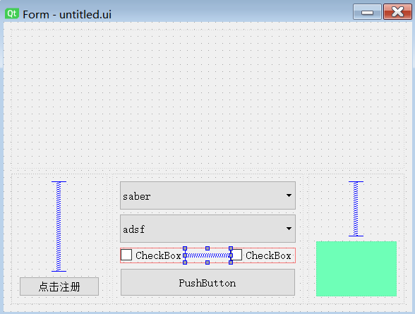
可以看到控件在对齐方面已经没有问题
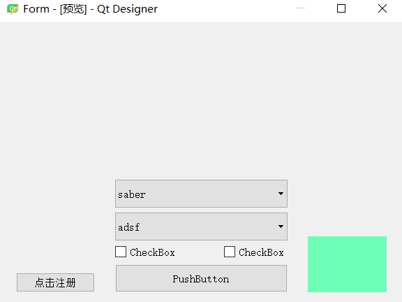
5.2.5 界面渲染
(只介绍按键功能,和本次项目无关,重新写时间太长了)
这里操作类似于html的css语法,如下:
1 | QWidget{ |
python加载css语法:
1 | with open("css/mainwindow.css","r") as file_css: |
结果显示:
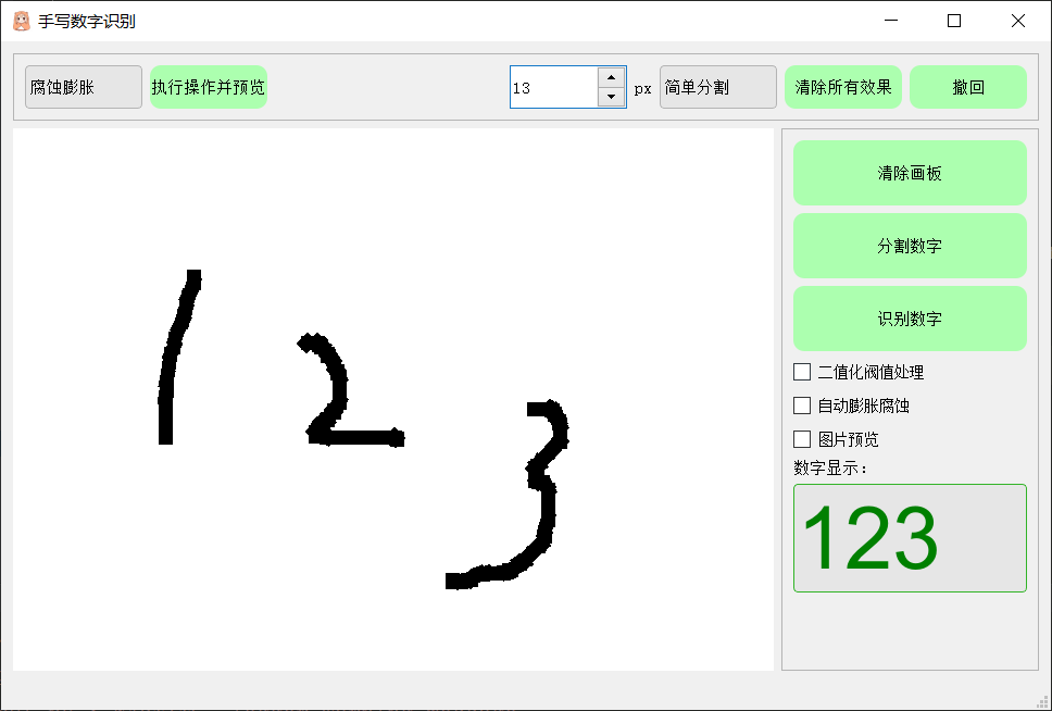
根据上面的原理,优化后的界面如下:
5.3 数字分割
5.3.1 简单分割
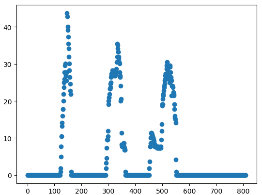
要实现数字识别,首先要对画板的数字进行分割,找到每个数字的位置。这里采用比较粗糙的识别方式,先对x方向的像素进行统计,统计图像如下,同理在对y方向进行统计,即可以得到每一个图像的位置。
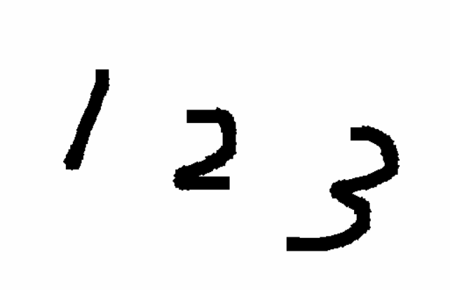
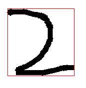
就是先确定x坐标,再确定y坐标,就可以定位数字的位置。定位到位置后添加padding后生成测试图片:
未添加padding的图片:
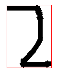
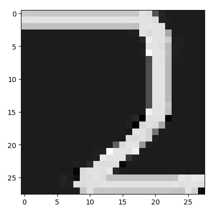
添加padding的图片:
思考:为什么要添加padding
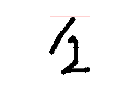
但是这种方法当数字挨的比较近之后,就会显示识别失误的问题,如下:
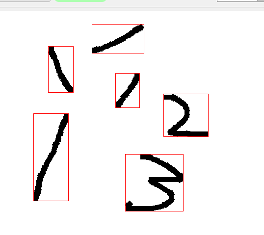
5.3.2 精确分割
- 图论遍历
类似于图论的遍历 - 深度优先遍历
程序使用递归,结构简单,好理解。但是当碰到较大的图的时候,递归深度过高会导致堆栈溢出。故而对于未知深度的递归程序不建议使用。 - 宽度优先遍历
可以解决深度优先遍历出现的问题。
深度优先遍历代码:
1 | def dfs(self, image, x, y): |
宽度优先遍历代码:
1 | def bfs(self, image, x, y): |
数字书写不再受到从左到右的限制
5.4 图像识别
见第4章
参考文献
1. LeNet-5详解 ↩