一、前言
说实话,没什么内容可写的,网络上面资料太多了,下面是整理:
tensorFlow社区:http://www.tensorfly.cn/ ,这个直接上神经网络有点看不懂。
知乎大佬:https://www.zhihu.com/question/49909565
TensorFlow入门:https://zhuanlan.zhihu.com/p/30487008 ,对TensorFlow基础知识讲解了一下
二、环境配置
有没有在为python的各种版本,各种库之间的依赖关系头痛不已。电脑上要同时按照python2.0~python3.* ,头不头痛,使用软件anaconda告别烦恼。 快速下载方法,参考工具目录IDM。
配置细节是:算了,太简单,不想写。
三、tensorFlow奇葩语法
tensorFlow其实不只是可以用来做神经网络,只要可以把数据转成流(不好形容)的形式,都可以使用tensorFlow帮你加速计算,从一些简单的例子开始。
3.1 定义变量
tensorFlow定义变量使用的是tf.Variable,从输出结果可以看到,w只是一个4字节的ref类型,在C语言上应该称之为指针,是一个引用,数据其实保存在tf内部。下面实现定义一个变量并且输出。
1 | import tensorflow as tf |
如果要把我定义的2打印出来怎么需要怎么操作?tensorFlow的使用机制和其他库有点不同,它把所有执行操作全部放在了tf.Session().run()里面,想要有实际运行/操作,全部靠这个run。那么接下来试试:
1 | import tensorflow as tf |
结果表明你在使用一个未初始化的变量,说明前面定义变量时,只是设置了一个句柄,下面还需要初始化操作。
注:使用with语法的好处是,它会自动调用tf.Session()的__enter__和__exit__,类似于C++的构造函数和析构函数,无需用户手动调用。
正确方法1
2
3
4
5
6
7
8
9
10
11import tensorflow as tf
w = tf.Variable(2,name="weight")
init = tf.initialize_all_variables()
with tf.Session() as sess:
sess.run(init)
print(sess.run(w))
结果:2
下面是不使用with的写法是:1
2
3
4
5
6
7
8
9
10
11
12
13
14
15
16import tensorflow as tf
w = tf.Variable(2,name="weight")
init = tf.initialize_all_variables()
try:
sess = tf.Session()
sess.run(init)
print(sess.run(w))
except:
print("error")
finally:
sess.close()
结果:2
3.2 线性回归代码详解
对所给值做线性回归,神经元是下面这个样子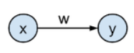
代码如下:1
2
3
4
5
6
7
8
9
10
11
12
13
14
15
16
17
18
19
20
21
22
23
24
25
26
27
28
29
30
31
32
33
34
35
36
37
38
39
40
41
42
43
44
45
46
47
48
49
50
51
52
53
54
55
56
57
58
59
60import tensorflow as tf # 神经网络库
import numpy #矩阵运算
import matplotlib.pyplot as plt # 用来绘图
rng = numpy.random
# Parameters
learning_rate = 0.01 #设置学习速率
training_epochs = 2000 #设置迭代次数
display_step = 50 #迭代50次,输出一次训练结果
# Training Data
train_X = numpy.asarray([3.3,4.4,5.5,6.71,6.93,4.168,9.779,6.182,7.59,2.167,7.042,10.791,5.313,7.997,5.654,9.27,3.1])
train_Y = numpy.asarray([1.7,2.76,2.09,3.19,1.694,1.573,3.366,2.596,2.53,1.221,2.827,3.465,1.65,2.904,2.42,2.94,1.3])
n_samples = train_X.shape[0] # 数据个数
# tf Graph Input
X = tf.placeholder("float") # 定义浮点型变量X,在这里并没有初始化,X其实是一个类似于句柄的东西
Y = tf.placeholder("float") # 定义浮点型变量Y,在这里并没有初始化
# Set model weights
W = tf.Variable(rng.randn(), name="weight") # 定义变量W,在这里并没有初始化
b = tf.Variable(rng.randn(), name="bias") # 定义变量b,在这里并没有初始化
# Construct a linear model
activation = tf.add(tf.mul(X, W), b) # 定义神经元计算方式X*W + b
# Minimize the squared errors
cost = tf.reduce_sum(tf.pow(activation-Y, 2))/(2*n_samples) #L2 loss # 定义代价函数
# 使用梯度下降算法,GradientDescentOptimizer,当然还有其他方法,minimize这个一般固定不变
optimizer = tf.train.GradientDescentOptimizer(learning_rate).minimize(cost) # 使用梯度下降算法
# Initializing the variables
init = tf.initialize_all_variables() # 定义初始化变量句柄,在这里其实还是没有开始初始化
# Launch the graph
with tf.Session() as sess:
sess.run(init) # 初始化之前设置的全部变量, (前面tf.Variable只是定义,没有初始化)
# Fit all training data
for epoch in range(training_epochs): # 循环迭代次数
for (x, y) in zip(train_X, train_Y): # 取出数据
sess.run(optimizer, feed_dict={X: x, Y: y}) # 开始学习,注意optimizer是之前定义好的方法
#Display logs per epoch step
if epoch % display_step == 0: # 没隔display_step次数,打印一次学习结果
print ("Epoch:", '%04d' % (epoch+1), "cost=", \
"{:.9f}".format(sess.run(cost, feed_dict={X: train_X, Y:train_Y})), \
"W=", sess.run(W), "b=", sess.run(b))
print ("Optimization Finished!") # 学习结束后输出结果
print ("cost=", sess.run(cost, feed_dict={X: train_X, Y: train_Y}), \
"W=", sess.run(W), "b=", sess.run(b))
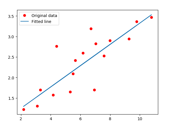
#画图
plt.plot(train_X, train_Y, 'ro', label='Original data')
plt.plot(train_X, sess.run(W) * train_X + sess.run(b), label='Fitted line')
plt.legend()
plt.show()
运行结束后效果:1
2
3
4
5
6
7
8
9
10
11
12
13
14
15
16
17
18
19
20
21
22
23
24
25
26
27
28
29
30
31
32
33
34
35
36
37
38
39
40
41
42Epoch: 0001 cost= 5.042386055 W= 0.93521166 b= -0.74453074
Epoch: 0051 cost= 0.219054163 W= 0.46031615 b= -0.71445704
Epoch: 0101 cost= 0.202640787 W= 0.44778362 b= -0.6242984
Epoch: 0151 cost= 0.188122705 W= 0.43599635 b= -0.5395013
Epoch: 0201 cost= 0.175281152 W= 0.42491 b= -0.45974758
Epoch: 0251 cost= 0.163922593 W= 0.4144832 b= -0.3847373
Epoch: 0301 cost= 0.153875872 W= 0.40467644 b= -0.3141882
Epoch: 0351 cost= 0.144989431 W= 0.3954529 b= -0.24783495
Epoch: 0401 cost= 0.137129351 W= 0.38677794 b= -0.1854279
Epoch: 0451 cost= 0.130177155 W= 0.3786189 b= -0.12673245
Epoch: 0501 cost= 0.124028035 W= 0.37094513 b= -0.071528085
Epoch: 0551 cost= 0.118589230 W= 0.3637278 b= -0.01960695
Epoch: 0601 cost= 0.113778725 W= 0.35693976 b= 0.029226175
Epoch: 0651 cost= 0.109524004 W= 0.3505553 b= 0.07515496
Epoch: 0701 cost= 0.105760820 W= 0.3445507 b= 0.118352175
Epoch: 0751 cost= 0.102432482 W= 0.3389031 b= 0.15898035
Epoch: 0801 cost= 0.099488728 W= 0.33359143 b= 0.19719209
Epoch: 0851 cost= 0.096885182 W= 0.32859573 b= 0.23313099
Epoch: 0901 cost= 0.094582528 W= 0.3238971 b= 0.26693237
Epoch: 0951 cost= 0.092546031 W= 0.31947792 b= 0.298724
Epoch: 1001 cost= 0.090744928 W= 0.3153215 b= 0.32862446
Epoch: 1051 cost= 0.089152046 W= 0.31141236 b= 0.3567465
Epoch: 1101 cost= 0.087743275 W= 0.30773562 b= 0.3831967
Epoch: 1151 cost= 0.086497456 W= 0.30427757 b= 0.40807357
Epoch: 1201 cost= 0.085395716 W= 0.3010253 b= 0.43147007
Epoch: 1251 cost= 0.084421404 W= 0.29796642 b= 0.4534753
Epoch: 1301 cost= 0.083559766 W= 0.29508942 b= 0.4741724
Epoch: 1351 cost= 0.082797796 W= 0.29238352 b= 0.49363872
Epoch: 1401 cost= 0.082124040 W= 0.28983864 b= 0.51194614
Epoch: 1451 cost= 0.081528224 W= 0.28744513 b= 0.5291656
Epoch: 1501 cost= 0.081001379 W= 0.28519377 b= 0.54536104
Epoch: 1551 cost= 0.080535494 W= 0.28307635 b= 0.5605937
Epoch: 1601 cost= 0.080123581 W= 0.28108492 b= 0.5749203
Epoch: 1651 cost= 0.079759359 W= 0.27921176 b= 0.58839536
Epoch: 1701 cost= 0.079437353 W= 0.2774501 b= 0.6010679
Epoch: 1751 cost= 0.079152651 W= 0.27579325 b= 0.6129879
Epoch: 1801 cost= 0.078900956 W= 0.27423516 b= 0.62419647
Epoch: 1851 cost= 0.078678481 W= 0.27276975 b= 0.63473856
Epoch: 1901 cost= 0.078481756 W= 0.27139154 b= 0.644654
Epoch: 1951 cost= 0.078307875 W= 0.27009517 b= 0.6539794
Optimization Finished!
cost= 0.07815707 W= 0.26889977 b= 0.6625798
致谢
感谢室友旺旺做的晚饭!!!居然还要我洗碗!